Trigonometric Regression#
Learning Objectives
Create linear regression models
Understand how to use a different basis (in this case, a trigonometric basis)
Apply a penalty to the regression model and learn about cross-validation
Learn about classically pulsating stars: this will enable you to determine exactly how bright a given pulsating star will be at any given time in the past or future! In addition, these statistical models we are fitting are a compact description of the lightcurve, which then enables us to compare observations of a star with a theoretical simulation. That in turn would enable us to determine things about the star, such as its mass, radius, metallicity, and age.
Introduction#
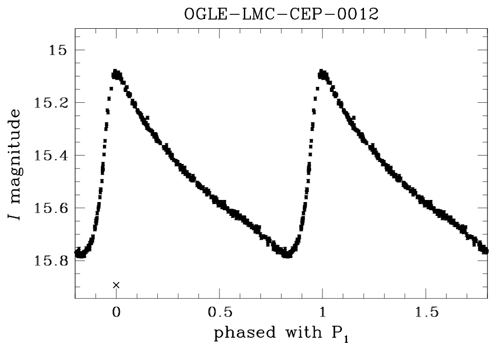
Classically pulsating stars such as Cepheids and RR Lyrae stars brighten and dim periodically.
Here is an example of a phased lightcurve obtained by the OGLE project of a Cepheid star in the Large Magellanic Cloud:
In this series of exercises, we will use linear regression to fit a trigonometric model to this phased lightcurve.
Lastly, we will use penalized regression for feature selection.
Review of Ordinary Linear Regression
Objective: Predict a dependent variable \(\mathbf{y}\) based on independent variables \(X\).
Model: \(\begin{align*} \mathbf{y} &= \beta_0 + \beta_1 X_1 + \beta_2 X_2 + \ldots + \beta_m X_m + \epsilon= \boldsymbol\beta \mathbf{X} + \epsilon \\ \end{align*}\)
where \(\beta_0\) is the intercept, \(\beta_1\) a coefficient, and \(\epsilon\) an error term.
Loss: \(\arg\min_{\boldsymbol\beta}||\mathbf{y} - \boldsymbol{\beta} \mathbf{X}||_2\)
Solution: \(\boldsymbol{\hat\beta} = (\mathbf{X}^\mathrm{T}\mathbf{X})^{-1}\mathbf{X}^\mathrm{T}\mathbf{y}\) (Thanks, Gauss!)
See also: https://scikit-learn.org/stable/modules/generated/sklearn.linear_model.LinearRegression.html
The Hubble Constant#
In this exercise we will use linear regression to derive \(H_0\). Below is the 1929 data from Edwin Hubble of Cepheid-host galaxies, which made him conclude that the Universe is expanding:
distances = np.array([0.21, 0.26, 0.27, 0.27, 0.45, 0.5, 0.8, 1.1, 1.4, 2.0]) # Mpc
velocities = np.array([130, 70, 185, 220, 200, 270, 300, 450, 500, 800]) # km/s
Exercise 1
Make a plot of velocity vs. distance
Obtain and plot the best fit line using ordinary linear regression (hint: use
sklearn)What Hubble constant does one find from these data? What does this imply about the age of the Universe, and how does this compare to modern values?
3D Linear Model#
In this exercise, we will practice generating data from a linear model (with noise) and visualizing it. We’ll then use the sklearn library to fit a linear model to the data.
Exercise 2
Generate random data according to the linear model
where \(x_1\) and \(x_2\) are uniform random variables, and \(\epsilon\) is a normal random variable.
Generate 100 data points according to this model.
Plot \(y\) vs \(x_1\) and \(y\) vs \(x_2\).
Make a 3D plot of these three variables. Visualize the data as points and the model as a plane. Extra credit: use ipywidgets to control the orientation of the 3D plot.
Use
sklearnto fit a linear model to your data.Add the plane of best fit to your 3D plot.
Cepheid Lightcurves#
We can now use the techniques we’ve practiced thus far to begin an investigation of the light curves (magnitude vs. time) of classically pulsating Cepheid stars.
Exercise 3
Download Cepheid data from the OGLE database: https://ogledb.astrouw.edu.pl/~ogle/OCVS/data/I/12/OGLE-LMC-CEP-0012.dat. (Backup/local link here)
Plot magnitude vs. time (with appropriate errorbars).
Plot magnitude vs. phase (with appropriate errorbars) by phasing the times according to the pulsation period of 2.6601839 days.
You should get something like this:
Trigonometric Regression#
Finally, we can apply trigonometric (a.k.a. sinusoidal) regression to investigate the relevant parameters of our Cepheids. A short review of the technique can be found in the dropdown.
Exercise 4
Fit a trigonometric linear regression model to the Cepheid observations
Plot the fitted model with the data
Use an ipython widget to adjust the number of parameters in the fit (and to update the plot)
Review of Trigonometric Regression
When dealing with periodic data, we can change our basis to
where
\(y\) is our (observed) timeseries
\(y_0\) is a mean value
\(t\) are the time points at which we have data
\(\omega\) is the main frequency of variability (assumed here to be known)
\(k\geq 1\) tells us how many terms are in our fit
and we fit for the amplitudes \(S,C\).
Note that if \(\omega\) is known, then \(y\) is linear in \(\mathbf{S, C}\).
Penalized Regressions#
It can be beneficial to regularize / penalize the fitting process. Here we will use two common methods: LASSO (L1) and Ridge (L2) regularization, and we’ll use cross-validation to determine the best penalty to choose. (For a review on cross-validation, see https://scikit-learn.org/stable/modules/cross_validation.html)
Exercise 5
Use a penalized regression model to fit the Cepheid data
Use an ipython widget to adjust the penalty (and to update the plot)
Use cross-validation to determine the optimal penalty (and plot it)
Review of Penalized Regression: LASSO (L1 Regularization)
a.k.a. least absolute shrinkage and selection operator
Objective: Eliminate less important features
Model: Add a penalty term \(\alpha \sum_{i=1}^{n} |\beta_i|\) to the loss function
Higher \(\alpha\) → more penalty → more coefficients set to zero
Loss: \(\arg\min_{\boldsymbol\beta}||\mathbf{y} - \boldsymbol{\beta} \mathbf{X}||_2 + \alpha \sum_{i=1}^{n} |\beta_i|\)
Solution: No closed form! Need to search.
Takehome message: LASSO completely eliminates some features.
https://scikit-learn.org/stable/modules/generated/sklearn.linear_model.Lasso.html
Review of Penalized Regression: Ridge (L2 Regularization)
a.k.a. Tikhonov regularization
Objective: Minimize the impact of less important features
Model: Add a penalty term \(\alpha \sum_{i=1}^{n} \beta_i^2\) to the loss function
Loss: \(\arg\min_{\boldsymbol\beta}||\mathbf{y} - \boldsymbol{\beta} \mathbf{X}||_2 + \alpha \sum_{i=1}^{n} \beta_i^2\)
where \(\alpha\) is a regularization penalty. Higher \(\alpha\) → more penalty → smaller coefficients
Solution: \(\boldsymbol{\hat\beta} = (\mathbf{X}^\mathrm{T}\mathbf{X} + \alpha \mathbf{I})^{-1}\mathbf{X}^\mathrm{T}\mathbf{y}\)
where \(\mathbf{I}\) is the identity matrix.
Takehome message: Ridge reduces the magnitude of coefficients, but doesn’t set them to zero.
https://scikit-learn.org/stable/modules/generated/sklearn.linear_model.Ridge.html
Exercise 6
Download the lightcurves of more Cepheids
Fit penalized regression models to them
Peform exploratory data analysis to find the relationships between the period, amplitudes, etc.